
Learn ML basics
Machine learning (ML) is a branch of computer science that applies various techniques to enable a computer to learn from data without substantial programming.
There are two ML types:
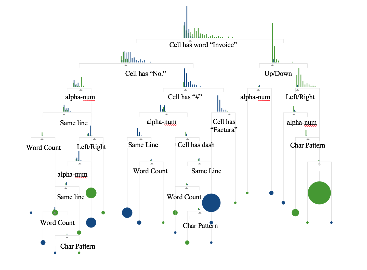
Supervised learning analyzes training data and produces an inferred function. The training data is a set of training examples. Each example is a pair consisting of an input object and a desired output value. Examples are logistic regression, a decision tree, a naive Bayes classifier, a support vector machine, bagging (random forest), some types of neural networks.
Unsupervised machine learning infers a function to describe a hidden structure from unlabeled data. Since the examples given to the learner are unlabeled, it is impossible to evaluate the accuracy of the structure produced by the relevant algorithm. This is one of the ways how you can distinguish unsupervised learning from supervised one. Examples are k-means, other types of neural networks.
Supervised learning
IA Cloud models are based on supervised ML algorithms that use training data to analyze hidden patterns and predict results based on their findings.
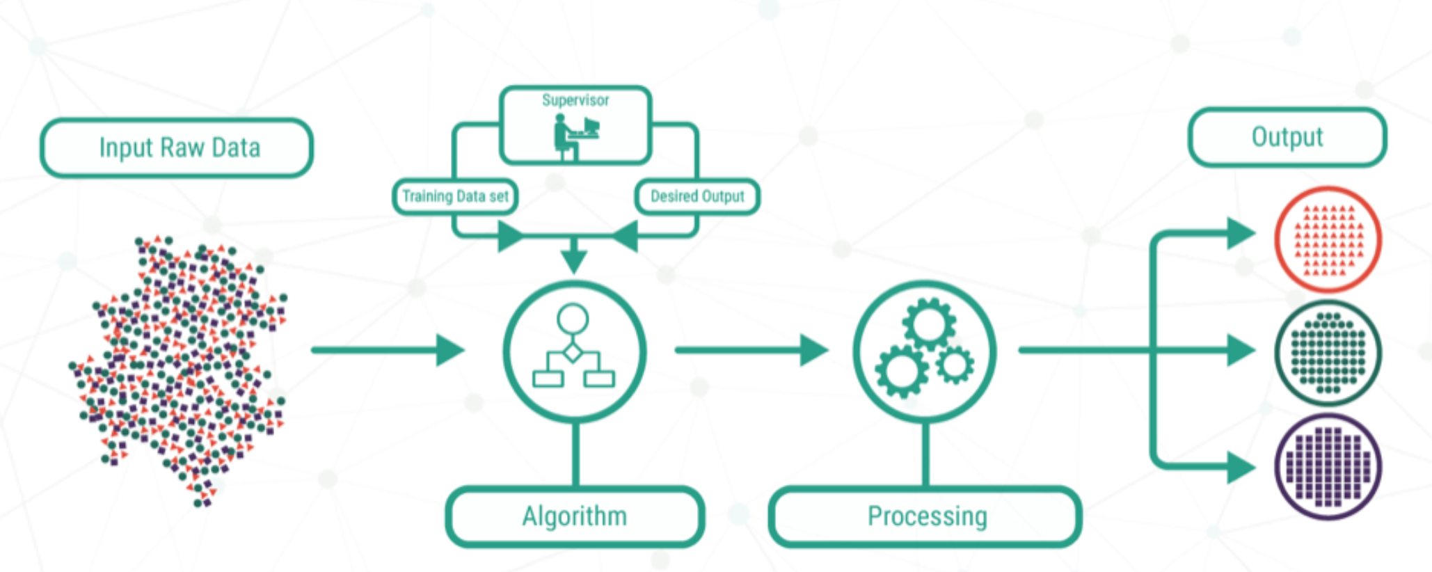
Building a supervised ML model usually includes the following steps:
Determine the type of objects to be used for training.
In IA Cloud, the most common problems are classification and information extraction. For classification, the object is a document-class pair. For information extraction, an object is a gold value-field pair. A gold value refers to the information to be extracted.
Collect the training set that represents how you can use the function in the real world.
In IA Cloud business cases, the human-in-the-loop approach is applied for supervision and consistent quality. Training sets are usually created by manually labeling documents for classification and gold values for information extraction. In rare cases, training sets are tagged automatically using provided historical data.
Determine the features that represent the learned function.
The model performance quality strongly depends on how input objects are represented. Typically, an input object is transformed into a feature vector containing features that describe the object. The number of these features should not be too large but should contain enough information to predict objects correctly. In IA Cloud out-of-the-box models, features are defined automatically, while in custom models—created manually.
Determine the structure of the learned function and the corresponding learning algorithm.
Complete the development phase (not required with IA Cloud out-of-the-box models).
Train the learning algorithm on an available training set and produce a model.
Evaluate the learned model performance.
Following the training process, evaluate the performance of the resulting model. To ensure the objectivity of evaluation, it is recommended to use a test set that is not a part of the training set.
The steps need to be completed for each case where ML is applied.
Let's see a simplified version of what model is using support vector machine (SVM) as an example. SVM is a binary classification algorithm. Given a set of objects belonging to two classes, it builds a function that divides objects accordingly in an n-dimensional feature space.
Let's assume you have a training set consisting of objects belonging to the red squares and blue circles classes. Our goal is to predict the class for a new unseen object.
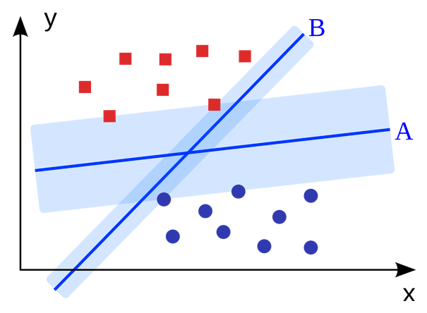
To solve the problem with SVM (a one-dimensional hyper-plane in the two-dimensional space), you need a training set of red squares and blue circles representative enough to describe all real-world objects of these classes. If the training set doesn't illustrate the real world adequately, the model trained on it can work incorrectly with the objects not included in the training set.
The next step is to define the features that describe each object and give information to build a function that can work correctly in the real world, not only on the training set. In IA Cloud, model features are generated automatically or created manually. In both cases, the whole training set is used as a source of features. Depending on various conditions, facts are transformed into features that describe objects and define each object's class.
Therefore, each object has some features. If you try to describe the objects from the picture below with two features, you get the following description:
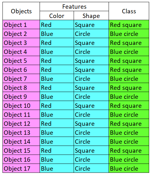
In IA Cloud AutoML, feature values are numeric, and each object is determined by the entirety of its feature values (the vector of features) and marked by a label (class).
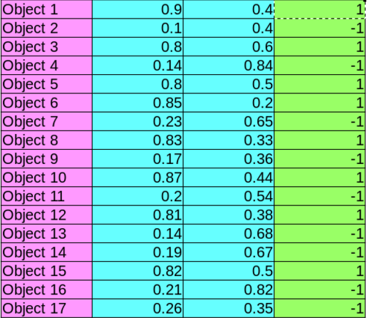
In this example (blue circles and red squares objects described by two features), all the objects are situated in the two-dimensional feature space, where each dimension corresponds to a certain feature. One object’s features define its coordinates.
In SVM, you define the object's class by the following function:
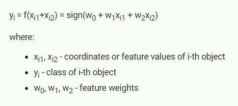
Feature weights are coefficients that show the importance of each feature and the strength of its impact on a classification decision. The class function returns 1 or -1 that defines which class is assigned to the object.
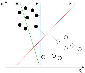
Now, you build a separating hyper-plane that divides objects into two classes. The process of building this function is a training process. There is more than one way to build a hyper-plane like this. The most optimal ones are as follows:
If the data set is linearly separable, the hyper-plane should classify all the objects correctly and with maximum margin (a red line on the picture).
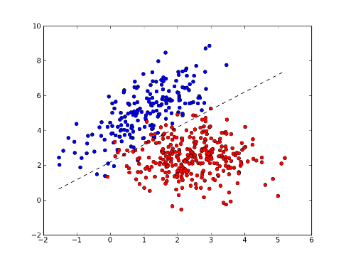
If the data set is not linearly separable, the number of incorrectly classified objects should be minimized.
A separating hyper-plane is described by the following formula:
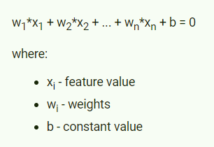
Feature values for objects in a data set are defined before the training starts. During the training process, SVM calculates feature weights and builds a separating hyper-plane. As mentioned before, there are many ways of building the hyper-plane.
Evaluate model
To define which way is better and the difference between them, evaluate how correctly they classify objects. To do that, run the model for some objects and check if they are classified correctly. If the data set is linearly separable, all the objects of one class should be on the same side of the hyper-plane.
Binary classification
Assume that both classes are equally interesting to you. For binary classification, there are four possible results:
Correctly classified red squares |
Incorrectly classified red squares |
|
|---|---|---|
Incorrectly classified blue circles |
Correctly classified blue circles |
Here, you need to separate correctly and incorrectly classified objects. They are true answers and false answers.
Objects of two classes are usually called positives (objects of the first class, for example, red squares) and negatives (objects of the second class, for example, blue circles):
- True positives (TP) and true negatives (TN) are objects of the first and second classes classified correctly.
- False positives (FP) and false negatives (FN) are objects of the first and second classes classified incorrectly. If you are more interested in one class, for example, you have an invoice or not invoice classification and want to process invoices (target class, relevant elements) further, the classification results look as follows:
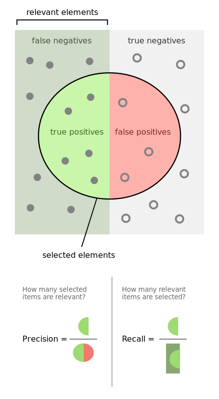
Their distribution in the table form is called a confusion matrix and looks like this:
TP |
FN |
|
|---|---|---|
FP |
TN |
Binary classification calculations
See binary classification calculations below:
| Formula | Description |
|---|---|
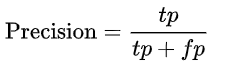 | Precision (calculated per class only) shows how exact the classification is: among all the objects defined by the model as red squares that actually belong to this class. It's calculated the following way: P = Correctly classified red squares or the total number of objects classified as red squares (the same for blue circles or any other class). |
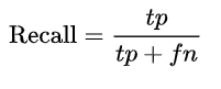 | Recall (calculated per class only) shows how complete the classification is: how many real red squares were classified as red squares. It's calculated the following way: R = Correctly classified red squares or the total number of all red squares in a data set (the same formula for blue circles or any other class). |
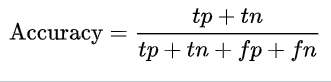 | Accuracy (calculated for the whole set) = Total number of correctly classified objects or the total number of objects. In the confusion matrix, it is the number of elements in diagonal. |
Multiclass classification of results
In the previous case of the binary classification, there were only two classes making the Positive class and the Negative one.
In the case of multiclass classification, there are two possible solutions of assigning the Positive or Negative, True or False relevance to classes:
- Define
trueorfalsevalues for each class separately (analyzes only TPs and FPs in the extracted class sample). - Set one class as a major one and treat the rest as an aggregated class—Others (negatives, irrelevant). The second method is used in IA Cloud more frequently.
Example 1 (first method)
Let's assume you have 30 documents belonging to three different classes: 10 documents of A-class, 10 documents of B-class, and 10 documents of C-class.
The algorithm processes them with the following results:
- 13 documents retrieved as A-class documents: 7 documents of A-class, 4 documents of B-class, and 2 documents of C-class
- 6 documents retrieved as B-class documents: 2 documents of A-class, 1 document of B-class, and 3 documents of C-class
- 11 documents retrieved as C-class documents: 1 document of A-class, 5 documents of B-class, and 5 documents of C-class
| Actual class | ||||
|---|---|---|---|---|
| A | B | C | ||
| Predicted class | A | True A | False A | False A |
| B | False B | True B | False B | |
| C | False C | False C | True C | |
| Actual class | ||||
|---|---|---|---|---|
| A | B | C | ||
| Predicted class | A | 7 | 4 | 2 |
| B | 2 | 1 | 3 | |
| C | 1 | 5 | 5 | |
The confusion matrix for example 1 looks as follows:
| A-class | B-class | C-class | |
|---|---|---|---|
| Precision | 7 / 13 = 53.8% | 1 / 6 = 16.7% | 5 / 11 = 45.45% |
| Recall | 7 / 10 = 70% | 1 / 10 = 10% | 5 / 10 = 50% |
Accuracy (for the whole set): only TP values are used in the numerator (documents which classes are recognized by the algorithm correctly), and all elements—in the denominator: Acc = 13 / 30 = 43.3%.
Example 2 (second method)
If you are focused on one class, for example, class A, you can transform your multiclass confusion matrix into the binary classification confusion matrix. In this case, you redraw the confusion matrix as follows:
| Actual class | ||||
|---|---|---|---|---|
| A | B | C | ||
| Predicted class | A | True Positive | False Positive | False Positive |
| B | False Negative | True Negative | True Negative | |
| C | False Negative | True Negative | True Negative | |
The other variant is as follows:
| Actual class | |||
|---|---|---|---|
| A | Other classes | ||
| Predicted class | A | True Positive | False Positive |
| Other classes | False Negative | True Negative | |
According to this, the confusion matrix for Example 2 looks like this:
| Actual class | |||
|---|---|---|---|
| A | Other classes | ||
| Predicted class | A | 7 | 6 |
| Other classes | 3 | 14 | |
- Precision = 7 / 13 = 53.8%
- Recall = 7 / 10 = 70%
- Accuracy = (7 + 14) / 30 = 70%
Information Extraction results
Information extraction models also classify their results as TPs, FPs, TNs, and FNs. The document is divided into tokens. In the beginning, each token is classified based on whether it should be extracted or not (positives and negatives).
Thus, the model finds the set of objects that can be extracted. There can also be additional conditions that the classified values should satisfy to be extracted. For example, you need one value for a field, and the model found five values that it considers suitable.
In this case, it can check which object has the maximum margin to the hyper-plane and chooses it–the object with the highest confidence or score. The margin describes how confident the model is in classifying the object as belonging to this class.
The IE model's quality is estimated by comparing gold data and extraction results received after applying a particular model.
To estimate a decision on an object, use the following metrics:
True positive: The value should be extracted and was extracted correctly (result = gold ≠ empty).
False positive: The value should not be extracted (gold = empty) but was extracted (result ≠ empty).
True negative: The value should not be extracted (gold = empty) and was not extracted (result = empty).
False negative: The value should be extracted (gold ≠ empty) but was not extracted by the model (result = empty).
False positive, False negative: One value should have been extracted, but the model extracted another (wrong) one. It consists of two parts:
- The model did not extract a correct value where the correct value was available; the machine missed the correct value—FN.
- The machine extracted a value, but the value was incorrect—FP.
caution
This mistake should be included into the FPs and FNs sets to get the correct statistics.
For examples, refer to the table below:
| Field name | Gold | Extracted | Decision |
|---|---|---|---|
invoice_date | 3/3/2022 | 3/3/2022 | True positive |
invoice_date | 5/2/2022 | False negative | |
invoice_date | 3/7/2022 | 3/3/2022 | False positive, False negative |
invoice_date | 9/5/2022 | False positive | |
invoice_date | True negative |
Typically, true negatives are not considered useful as customers are usually interested only in objects that should be extracted.
There is a slight difference between estimating classification and information extraction results. In classification, the number of classified objects and the total number of objects are the same. In the case of an information extraction task, imagine you need to process 1,000 documents, and only 500 of them contain a gold value for a certain field (for example, an email). Let's assume your model extracted 400. The result is as follows: the number of documents ≠ the number of gold values ≠ the number of extracted values.
Hence, in contrast to classification tasks, you have two new metrics you are interested in:
- How many objects you should extract (Gold values).
- How many objects you extracted (extracted values).
To know how accurately the model extracts values, calculate Precision:
- Precision (P) = Correctly extracted / Extracted, or
- Precision (P) = TP / (TP + FP), where: FP + (FP, FN) ∈ FP
To know the percent of the existing values that can be extracted by the model, calculate Recall:
- Recall (R) = Correctly extracted / Gold values, or
- Recall (R) = TP / (TP + FN), where: FN + (FP, FN) ∈ FN
The accuracy is not used for information extraction as it describes how accurate the model is for all the classes, while you have two classes (empty values and not empty values) in information extraction. You are usually interested in quality metrics of not empty values only.
Let's see how it works with our documents with emails. You have:
| Number of documents | Gold values | Extracted values | TP (correctly extracted) | FP (model's mistakes) | FN (missed gold values) |
|---|---|---|---|---|---|
| 1000 | 500 | 400 | 350 | 50 | 150 |
- P = TP / Extracted = 350 / 400 = 0.875 = 87.5%
- R = TP / Gold = 350 / 500 = 0.7 = 70%
Natural Language Processing
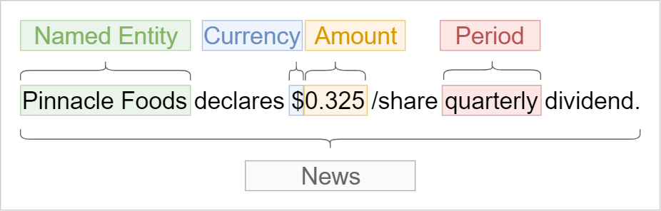
Given: unstructured text (dividend news, invoices, reports)
Task: extract particular fields (invoice number, date, amount, currency) from this unstructured text using ML.
Phase 1: Annotation (tagging)
Phase 2: Feature extraction
A sample set of Features for the Amount field is as follows:
| Feature | Value |
|---|---|
| is a number | Yes |
| position after the Currency field | Yes |
| position before "/share" | Yes |
| can be less than zero | No |
| is the last word in a sentence | No |